The most common way to plan purchasing in e-commerce looks like this: take sales from the last 30, 60, or 90 days, compute the average, and multiply by the number of days until your next delivery. Simple, fast, built into Excel and most ERPs. The problem is that this method isn't wrong occasionally and by a little — it's wrong systematically, and most of all exactly when the stakes are highest.
To see why, you first have to understand what a forecast actually is.
Demand isn't one number — it's several patterns stacked on top of each other
Every product's sales can be broken down into components. The forecasting literature (including MIT's SCM program materials) describes four:
- Level — the baseline volume, "what normally sells."
- Trend — whether the level is rising or falling over time.
- Seasonality — a repeating, calendar-driven pattern (December, Valentine's Day, back-to-school).
- Noise — random fluctuation you can't predict and shouldn't try to.
A good forecast separates signal from noise: it captures level, trend, and seasonality, and ignores the noise. A plain average does the opposite — it blends all four into a single, lagging number. That's why it loses in three typical situations. Here's each one, with numbers.
1. Trend: the average always looks backward
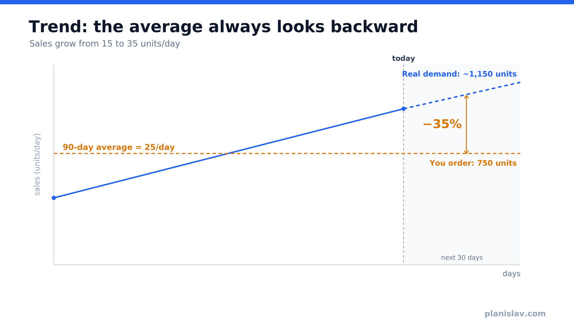
Take a product that grows steadily: 90 days ago it sold ~15 units/day, today it sells ~35 units/day.
The 90-day average = 25 units/day. Looks reasonable. But that's the midpoint of a period that's already gone. If the trend holds, over the next 30 days sales will average ~38 units/day.
- You order to the average: 25 × 30 = 750 units.
- Real demand: 38 × 30 ≈ 1,150 units.
- You're short ~400 units — nearly 35% of demand.
The average always drags you back to a lower, past level. On growing products you chronically under-order (and fight stockout fires); on declining ones you chronically over-order (and sink cash). The longer the window (90 vs 30 days), the worse it gets, because the average reaches even further into the past.
2. Seasonality: the average is blind to the peak
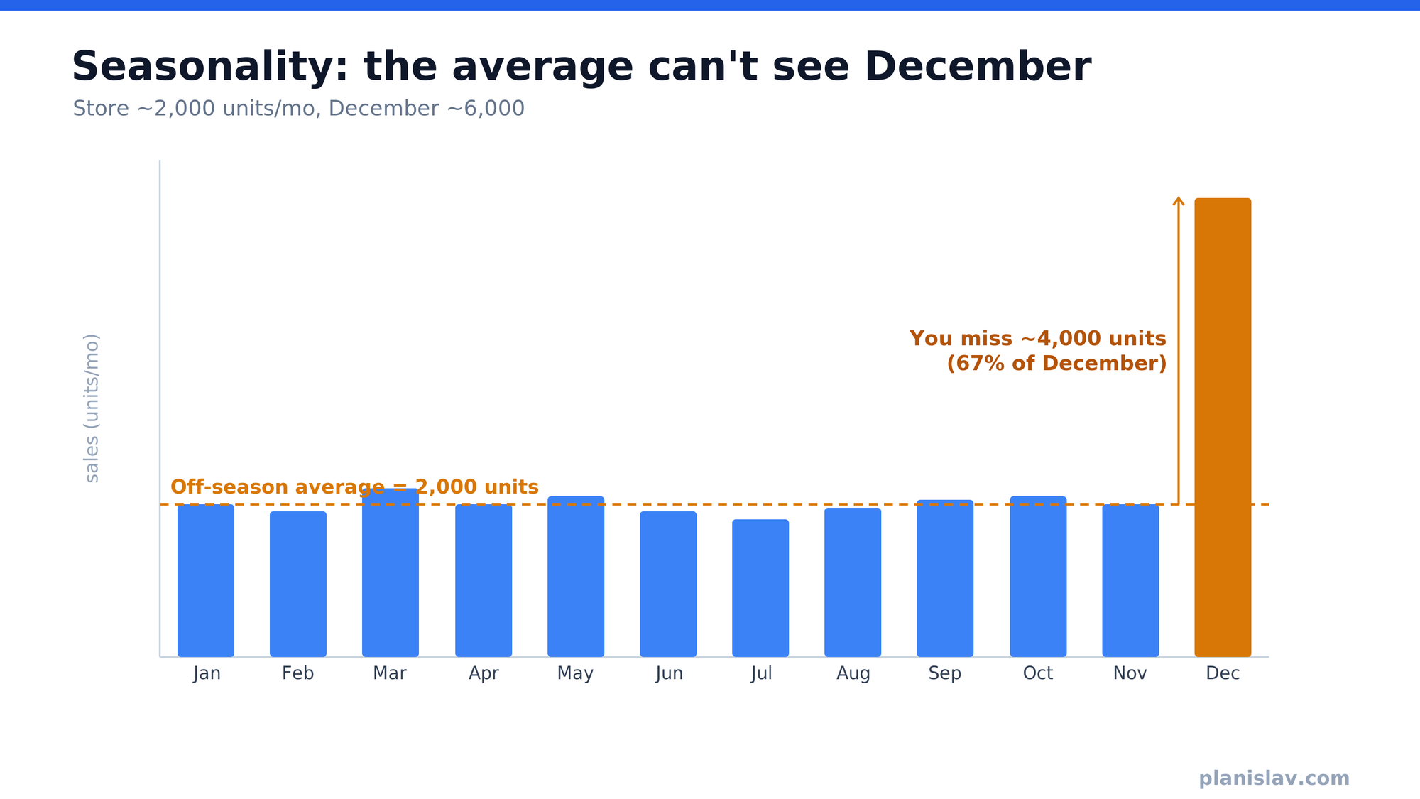
This is where it gets expensive. Take a store that sells ~2,000 units/month most of the year, but ~6,000 units in December — three times more. (This isn't a made-up example; in the data we use to test our engine, the December peak really does exceed three times a normal month.)
In November you compute the 90-day average. It covers August–October — off-season months, ~2,000 units. You order for December like a normal month:
- You order: ~2,000 units.
- Real December demand: ~6,000 units.
- You fail to sell ~4,000 units — 67% of December's demand — precisely when the whole year's profit is made.
The opposite problem hits in January. Now your 90-day average includes the December peak and jumps to ~3,300 units/month. You carry that inflated level into dead January and February and over-order by ~1,300 units per month.
The key point: a rolling average forces you to choose — either you react to current changes, or you see seasonality. You can't have both at once. A short window (30 days) is responsive but has no idea December is coming. A long window (90 days) smooths, but smears the peak across months that don't need it. Seasonality detection solves this differently: it assigns December a seasonal factor (say ×3) and plans the peak before it arrives — while staying responsive to the current level.
3. Intermittent demand: the average describes a day that never happens
Most of an e-commerce catalog is the long tail — SKUs that sell rarely and unevenly. That's not the exception, it's the norm. And here the average isn't so much imprecise as misleading.
A product sold on only 6 days out of 90, ~50 units each time. That's 300 units total. Average = 300 / 90 = 3.33 units/day.
Except no day looks like 3.33 units. For 84 days sales are zero, and on 6 days they're ~50. If you set stock "to the average" (~3/day), the first real batch of 50 wipes you out; the rest of the time you sit on stock that doesn't move. Smoothing this kind of demand with a plain average, as MIT puts it, "just adds noise."
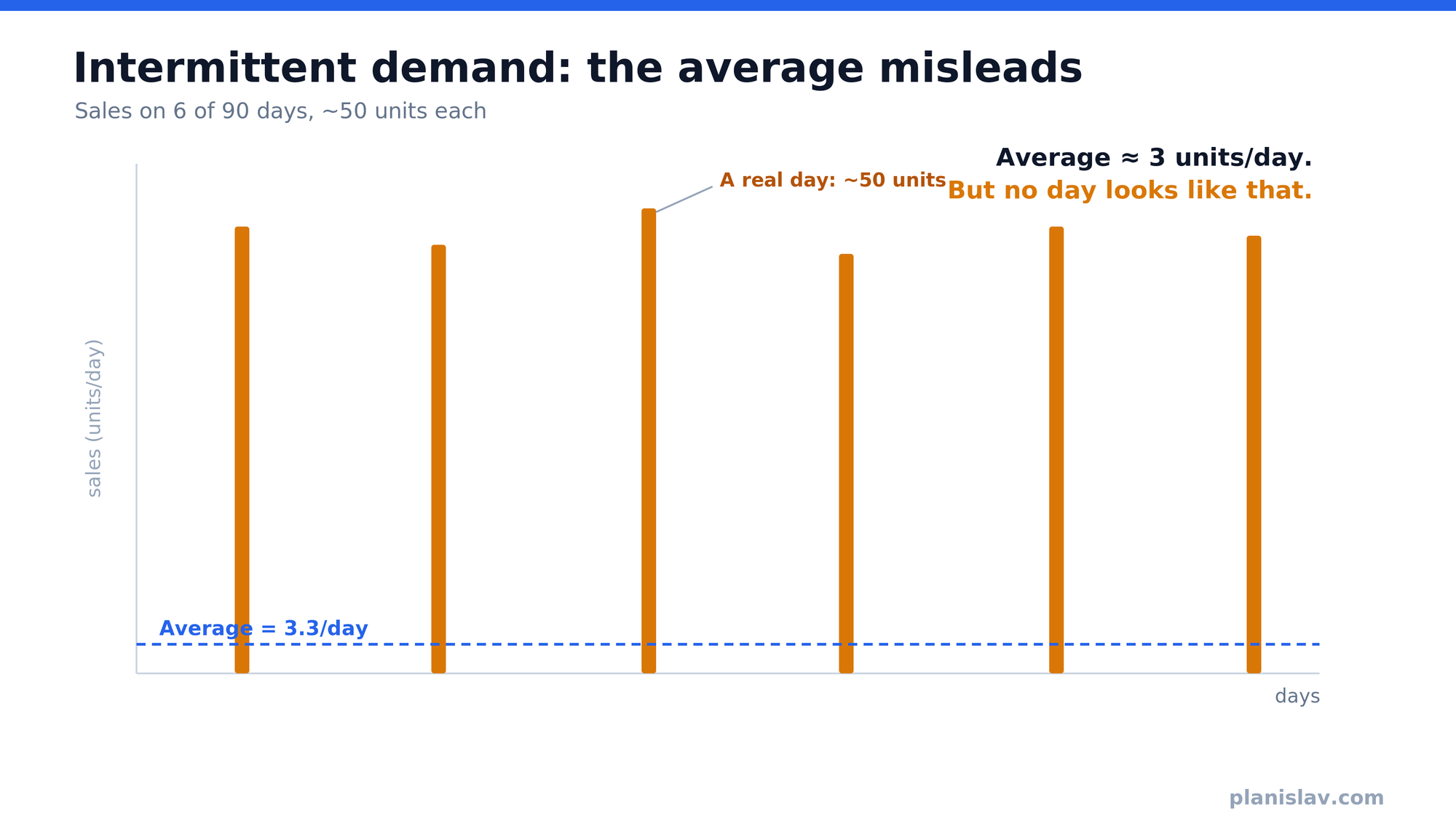
The right approach (Croston's method) splits two separate questions: how big is a typical order (size ≈ 50) and how often does it arrive (every ~15 days). The demand rate is 50/15 ≈ 3.33/day — the same average! — but now you know you must cover a single hit of 50 units, not 3 units a day. Same number, completely different purchasing decision.
A few concepts worth knowing
- Level, trend, seasonality, noise — the four components of any sales series (above).
- Seasonal factor — how far a given month/week deviates from normal (December ×3 = three times the average).
- Intermittent / lumpy demand — sales in rare, uneven batches; dominates the e-commerce long tail.
- Cold start — a new SKU with no history. The average fails here by definition: there's nothing to average. In e-commerce this is a permanent problem (new products weekly), not an incident.
- Responsiveness vs seasonality — the trade-off a plain average forces on you, and one you don't have to accept.
Why seasonality in particular is hard (and matters most)
Detecting seasonality isn't the same as "drawing bars by month." You have to answer three questions: does the pattern actually repeat year over year (rather than being a one-off coincidence), how strong is it, and which SKUs ride the whole-business rhythm versus having their own micro-season. In real data you can see that alongside the main December peak, separate groups emerge: products peaking at Valentine's Day, at Women's Day, at Mother's Day. A plain average sees none of them. A tool that recognizes them plans purchasing for each of those peaks ahead of time — instead of chasing them after the fact.
Summary
A 30/60/90-day average isn't "a slightly worse forecast." It's a method that by design lags the trend, is blind to the season, and misreads intermittent demand — meaning it fails in exactly the three places where inventory hurts most. Forecasting means breaking sales down into components and computing each one separately: level, trend, and seasonality apart, and the noise in the bin.
Where Planislav comes in
Planislav does this for you — with nothing to configure. It analyzes your sales history, detects seasonality on its own (both the global pattern and individual products' micro-seasons), and combines it with responsiveness to the current level — giving you what a plain average can't: both at once. The output isn't charts to interpret or sliders to tweak, but a purchase list: buy X units by day Y from supplier Z.
Stop guessing how much to order. — planislav.com
Sources I rely on: MIT SCM program materials (MicroMasters in Supply Chain Management), Nicolas Vandeput's work on forecasting and intermittent demand, Croston's method, and research on e-commerce demand forecasting (including the M5 competition).